前言
植物的分子遗传研究的重要优势在于遗传群体的易得性。通过设计杂交混合不同来源亲本的基因组,自交获得一系列基因型和表型存在分离的作图群体。但生产上不依赖种子繁殖的高等植物基因组上往往具有较高的杂合率,且具有强的自交不亲和性,如土豆和柑橘。一般利用两个高度杂合的双亲杂交,构建杂种一代群体,用于育种和遗传分析。
Lep-Map3是一款新颖免费的遗传作图软件,支持大量标记和个体的遗传图谱构建,尤其是低测序深度的全基因组测序数据。
数据准备
系谱
系谱文件包含样本名及家系等相关信息,以tab为分隔符,示例如:
| CHR | POS | F | F | F | F | F | F | F |
|---|---|---|---|---|---|---|---|---|
| CHR | POS | SYH | ZNX | F1 | F10 | F101 | F103 | F104 |
| CHR | POS | 0 | 0 | ZNX | ZNX | ZNX | ZNX | ZNX |
| CHR | POS | 0 | 0 | SYH | SYH | SYH | SYH | SYH |
| CHR | POS | 2 | 1 | 0 | 0 | 0 | 0 | 0 |
| CHR | POS | 0 | 0 | 0 | 0 | 0 | 0 | 0 |
line1:家系名称,可多父母多家系
line2:样本名称
line3:父本名称,对应第二行第四列
line4:母本名称,对应第二行第三列
line5:性别,1为male,2为female,0为unknow
line6:表型,用不到,全为0
基因型
VCF文件,必须包含likelihood信息,使用vcftools注意增加–recode-INFO-all参数。
从GATK的基因型文件,主要处理步骤为
- 提取SNP
- GATK硬过滤
- Founder多态性变异鉴定
- offspring高质量变异鉴定
- ParentCall2格式转换
GATK提取SNP
singularity exec -e ~/Singularity_lib/gatk-4.2.2.0.sif gatk SelectVariants
-R ~/wpf/Datasets/Reference/Lychee/BWA/Lchinesis_genome.fa
-V ../07.VCF/raw/pop.vcf.gz
-O ../07.VCF/variant/pop.snp.vcf.gz
--select-type-to-include SNP
GATK硬过滤
singularity exec -e ~/Singularity_lib/gatk-4.2.2.0.sif gatk VariantFiltration
-R ~/wpf/Datasets/Reference/Lychee/BWA/Lchinesis_genome.fa
-V ../07.VCF/variant/pop.snp.vcf.gz
--filter-name "firstFilter"
--filter-expression "QD < 2.0 || MQ < 40.0 || FS > 60.0 || SOR > 3.0
|| MQRankSum < -12.5 || ReadPosRankSum < -8.0"
-O ../07.VCF/gatkvf/pop.snp.filt.vcf.gz
Founder多态性变异鉴定
- 初过滤标准为PASS,二等位,无缺失,测序深度为平均测序深度的一半至两倍
vcftools
--gzvcf pop.snp.filt.vcf.gz
--remove-filtered-all
--indv founder1
--indv founder2
--max-alleles 2
--min-alleles 2
--max-missing 1
--max-meanDP 60
--min-meanDP 15
--recode
--out founder- 多态性具有重组信息的标记筛选,即至少有一个亲本为杂合型
import re
vcf = open('founder.recode.vcf')
output = open('founder.filter.vcf','w')
for i in vcf:
    try:
        row = re.split(r'\t',i)
        p1 = re.split(r'\:',row[9])[0]
        p2 = re.split(r'\:',row[10])[0]
        if (p1 == '0/1' or p2 == '0/1'):
            output.write(i)
        else:
            continue
    except IndexError:
        output.write(i)
vcf.close()
output.close()- 高质量位点筛选,SNPable筛选出无重复比对的位点
awk '{print$1"\t"$2}' founder.filter.vcf |grep -v "#" > founder.pos
apply_mask_l mask_35_50.fa founder.pos > foundermask.pos
offspring高质量变异鉴定
- 初过滤标准为缺失率,maf和founder高质量位点
vcftools
--gzvcf pop.snp.filt.vcf.gz
--max-missing 0.8
--maf 0.05
--positions foundermask.pos
--recode-INFO-all
--recode
--out offspring_poly- 分割染色体
vcftools
--vcf offspring_poly.recode.vcf
--chr Chr1
--recode-INFO-all
--recode
--out Chr1
ParentCall2格式转换
输入为十进制文件,压缩文件会导致读取出错
java -cp ~/software/LepMAP3/bin/ ParentCall2
data=pedigree.txt
vcfFile=Chr1.recode.vcf
removeNonInformative=1 > Chr1.call
Filtering2过滤偏分离标记
java -cp ~/software/LepMAP3/bin/ Filtering2
data=Chr1.call
removeNonInformative=1
dataTolerance=0.001 > Chr1_chisq.call
无参标记的遗传图谱构建
无参考基因组项目没接触过,或许GBS或RADseq可以产生这些标记。标记鉴定的基本思路应该是聚类测序read,组装或不组装生成参考序列(以每一种read为独立的参考序列)并鉴定标记,这些标记没有确切的坐标,通过后代的分离重组情况,重建遗传连锁图,确定标记间的相对位置。
基本流程为
- SeparateChromosomes2标记分群
- JoinSingles2All单独标记插补进连锁群
- OrderMarkers2标记排序,计算遗传距离
分群
java -cp ~/software/LepMAP3/bin/ SeparateChromosomes2
data=Chr1_chisq.call
lodLimit=5
numThreads=8
distortionLod=1 > Chr1_chisq.map
插补
java -cp ~/software/LepMAP3/bin/ JoinSingles2All
map=Chr1_chisq.map
data=Chr1_chisq.call
distortionLod=1
numThreads=8
lodLimit=4
iterate=1 > Chr1_chisq_js_iterated.map
排序
java -cp ~/software/LepMAP3/bin/ OrderMarkers2
numThreads=20
map=Chr1_chisq_js_iterated.map
data=Chr1_chisq.call > Chr1_chisq.order
计算遗传距离
java -cp ~/software/LepMAP3/bin/ OrderMarkers2
evaluateOrder=Chr1_chisq.order
data=Chr1_chisq.call
improveOrder=0
sexAveraged=1 > Chr1_chisq_sexAve.order

java -cp ~/software/LepMAP3/bin/ OrderMarkers2
evaluateOrder=Chr1_chisq.order
data=Chr1_chisq.call
improveOrder=0 > Chr1_chisq_sex.order
有参标记的遗传图谱构建
有参考基因组的标记无需分群排序,按照物理位置的顺序直接计算重组距离。
标记数量过多,以10kb为window构建遗传连锁图,主要流程为
- 构建10kb binning图谱
- OrderMarkers2排序
- 提取window代表基因型
- OrderMarkers2计算遗传距离
binning
awk 'BEGIN{print "#binned markers"}(NR>7)
{if (prevc != $1 || $2-prevp >= 10000) {++n;prevp=$2;prevc=$1}; print n}'
Chr1_chisq.call > Chr1_chisq.map
排序
java -cp ~/software/LepMAP3/bin/ OrderMarkers2
numThreads=20
map=Chr1_chisq.map
data=Chr1_chisq.call
recombination1=0
recombination2=0
outputPhasedData=4 > Chr1_chisq.order
提取标记
利用脚本order2data.awk提取binning标记
#script for marker binning...
BEGIN{
#ACxAG=AA,AC,AG,CG
        map["AA"] = "1 0 0 0 0 0 0"#00
        map["AC"] = "0 1 0 0 0 0 0"#01
        map["AG"] = "0 0 1 0 0 0 0"#10
        map["CG"] = "0 0 0 0 0 1 0"#11

        if (chr == "")
                 chr = 1
}
/^[^#]/{
        for (j = 7; j <= NF; ++j)
                if ($j ~ /#$/) {
                        $j = substr($j, 1, length($j) - 1)
                        oldNF = j
                        break
                }
        if (oldNF == NF)
                next
        if (prev == "" && pedigree) {
                s1 = "CHR\tPOS"
                s2 = "CHR\tPOS"
                s3 = "CHR\tPOS"
                s4 = "CHR\tPOS"
                s5 = "CHR\tPOS"
                s6 = "CHR\tPOS"
                f = 1
                nt = 0
                for (j = 7; j <= oldNF; j+=3) {
                        n = length($j) / 2
                        s1 = s1 "\tF" f "\tF" f
                        s2 = s2 "\t" (nt + 1) "\t" (nt + 2)
                        s3 = s3 "\t0\t0"
                        s4 = s4 "\t0\t0"
                        s5 = s5 "\t1\t2"
                        s6 = s6 "\t0\t0"
                        for (i = 1; i <= n; ++i) {
                                s1 = s1 "\tF" f
                                s2 = s2 "\t" (nt + i + 2)
                                s3 = s3 "\t" (nt + 1)
                                s4 = s4 "\t" (nt + 2)
                                s5 = s5 "\t0"
                                s6 = s6 "\t0"
                        }
                        nt += n + 2
                        ++f
                }
                print s1 "\n" s2 "\n" s3 "\n" s4 "\n" s5 "\n" s6
        }

        s = ""
        nt = 0
        for (j = 7; j <= oldNF; j+=3) {
                s = s "\t" map["AC"] "\t" map["AG"]
                n = length($j) / 2
                for (i = oldNF + nt + 1; i <= oldNF + nt + 4 *n; i+=4)
                        s = s "\t" $i " " $(i+1) " " $(i+2) " 0 0 " $(i+3) " 0"
                nt += 4 * n
        }
        if (prev != s || FILENAME != prevFN)
                print $1 "\t" chr s
        prev = s
        prevFN = FILENAME
}
awk -vfunnData=1 -f order2data.awk ../02.Orderraw/Chr1_chisq.order |
awk '{print$1}' > Chr1_chisq.index
awk '{print$1"\t"$2}' Chr1_chisq.call |grep Chr1 > Chr1_chisq.poslibrary(tidyverse)
pos <- read_tsv("Chr1_chisq.pos", col_names = FALSE) %>%
mutate(id = row_number())
index <- read_tsv("Chr1_chisq.index", col_names = FALSE) %>%
rename(id = X1)
tmp <- index %>%
left_join(pos, by = "id") %>%
select(-id)
write_tsv(tmp, file = "Chr1_chisq_bin.pos", col_names = FALSE)vcftools
--vcf Chr1_chisq.recode.vcf
--positions Chr1_chisq_bin.pos
--recode
--recode-INFO-all
--out Chr1_chisq_bin
java -cp ~/software/LepMAP3/bin/ ParentCall2
data=pedigree.txt
vcfFile=Chr1_chisq_bin.recode.vcf > Chr1_chisq_bin.call计算遗传距离
awk '{print NR}' Chr1_chisq_bin.pos > Chr1_chisq_bin.order

java -cp ~/software/LepMAP3/bin/ OrderMarkers2
evaluateOrder=Chr1_chisq.order
data=Chr1_chisq.call
improveOrder=0
sexAveraged=1 > Chr1_chisq_sexAve.order

java -cp ~/software/LepMAP3/bin/ OrderMarkers2
evaluateOrder=Chr1_chisq.order
data=Chr1_chisq.call
improveOrder=0 > Chr1_chisq_sex.order
转换基因型
- 利用脚本map2genotypes.awk转换基因型。
#converts phased data to "genotypes"
#usage:
#java ... OrderMarkers2 ... outputPhasedData=1 > order_with_phase_LM3.txt
#awk [-vchr=X] [-vfullData=1] -f map2genotypes.awk order_with_phase_LM3.txt
#output columns marker name, chr, male postion, female postion, genotypes coded as "1 1", "1 2", "2 2" and 0 as missing
#providing fullData ouputs parents and pedigree...
BEGIN{
        map["00"]="1 1"
        map["01"]="1 2"
        map["10"]="2 1"
        map["11"]="2 2"
        map["0-"]="1 0"
        map["-0"]="0 1"
        map["-1"]="0 2"
        map["1-"]="2 0"
        map["--"]="0 0"
        if (chr == "")
                chr = 0
}
(/^[^#]/){
        if (!notFirst && fullData){
                notFirst = 1
                s1 =  "MARKER\tCHR\tMALE_POS\tFEMALE_POS"
                s2 =  "MARKER\tCHR\tMALE_POS\tFEMALE_POS"
                s3 =  "MARKER\tCHR\tMALE_POS\tFEMALE_POS"
                s4 =  "MARKER\tCHR\tMALE_POS\tFEMALE_POS"
                s5 =  "MARKER\tCHR\tMALE_POS\tFEMALE_POS"
                s6 =  "MARKER\tCHR\tMALE_POS\tFEMALE_POS"
                for (i = 7; i<=NF; i+=3) {
                        n = length($i) / 2
                        p1 = "P" (++numParents)
                        p2 = "P" (++numParents)
                        s1 = s1 "\t" p1 "x" p2 "\t" p1 "x" p2
                        s2 = s2 "\t" p1 "\t" p2
                        s3 = s3 "\t" 0 "\t" 0
                        s4 = s4 "\t" 0 "\t" 0
                        s5 = s5 "\t" 1 "\t" 2
                        s6 = s6 "\t" 0 "\t" 0
                        for (j = 1; j <= n; ++j) {
                                s1 = s1 "\t" p1 "x" p2
                                s2 = s2 "\tC" (++numOffspring)
                                s3 = s3 "\t" p1
                                s4 = s4 "\t" p2
                                s5 = s5 "\t0"
                                s6 = s6 "\t0"
                        }
                }
                print s1
                print s2
                print s3
                print s4
                print s5
                print s6
        }
        s = $1 "\t" chr "\t" $2 "\t" $3
        for (i = 7; i<=NF; i+=3) {
                if (fullData) #parental data
                        s = s "\t1 2\t1 2"
                n = length($i) / 2
                p1 = substr($i,1,n)
                p2 = substr($i,n+1)
                for (j = 1; j <= n; ++j)
                        s = s "\t" map[substr(p1, j, 1) substr(p2, j, 1)]
        }
        print s
}
awk -vfullData=1 -f map2genotypes.awk Chr1_chisq_sex.order >
Chr1_chisq_sex.geno
awk -vfullData=1 -f map2genotypes.awk Chr1_chisq_Avesex.order >
Chr1_chisq_sexAve.geno- 去除重负和偏分离位点,符合GACD输入标准
geno <- fread("Lychee/Output/geno.tsv") %>%
  as_tibble() %>%
  mutate(chrom = sapply(str_split(marker, "_"), `[`, 1))

# 去除重复
tmp <- geno %>%
  unite(col = "sig", names(select(., starts_with("F"))), sep = "-", remove = FALSE) %>%
  mutate(leadsig = lead(sig, default = "0"))  %>%
  group_by(chrom) %>%
  filter(sig != leadsig) %>%
  select(marker, chrom, pos, starts_with("F"))

# 去除极端偏分离位点
tmp2 <- tmp %>%
  rowwise() %>%
  mutate(t = length(unique(c_across(cols = starts_with("F"))))) %>%
  filter(t > 1) %>%
  select(-t)
作图
遗传连锁图
利用R/qtl包来绘制中性遗传连锁图谱
suppressWarnings(suppressMessages(library(tidyverse)))
suppressWarnings(suppressMessages(library(qtl)))
suppressWarnings(suppressMessages(library(data.table)))
suppressWarnings(suppressMessages(library(ggprism)))

path <- "C:/Users/wpf/Desktop/project/Bipgenetic/"

file <- fs::dir_ls(path = str_c(path, "Lychee/Data/geno/"), glob = "*Ave*")

tmp <- map_dfr(.x = file,
               .f = ~ read_tsv(.,
                               skip = 1,
                               col_select = c(1:4),
                               show_col_types = FALSE),
               .id = "Chrtmp")

tmp2 <- tmp %>%
  filter(MARKER != "MARKER") %>%
  mutate(chrom = sapply(str_split(str_replace(Chrtmp, path, ""), "/|_"), `[`, 4),
         markername = str_c(chrom, "-", MARKER),
         chr = str_sub(chrom, 4) %>% as.numeric(),
         pos = as.numeric(MALE_POS)) %>%
  select(markername, chr, pos) %>%
  arrange(chr) %>%
  column_to_rownames(var = "markername")

map <- table2map(tmp2)
plot.map(map)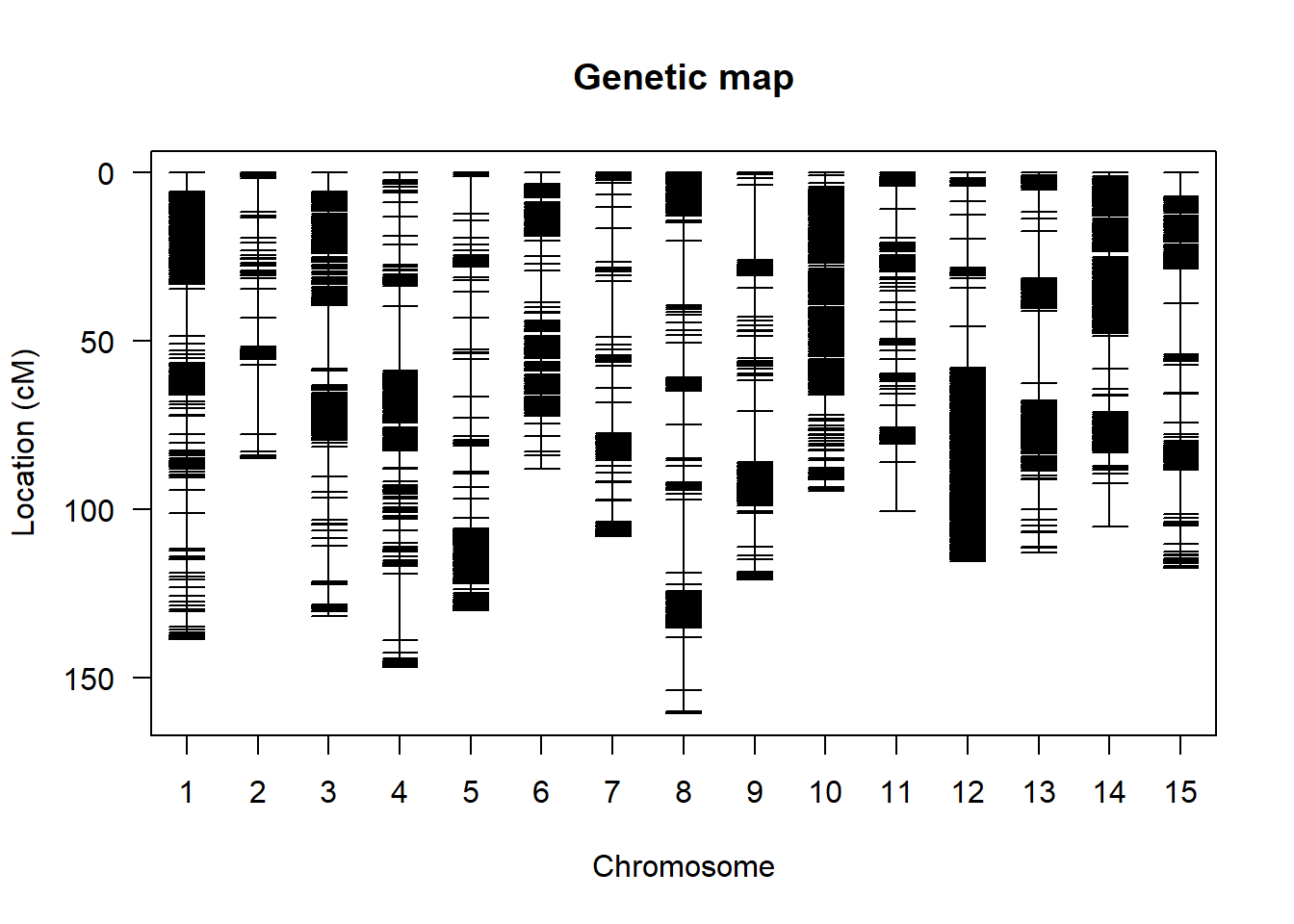
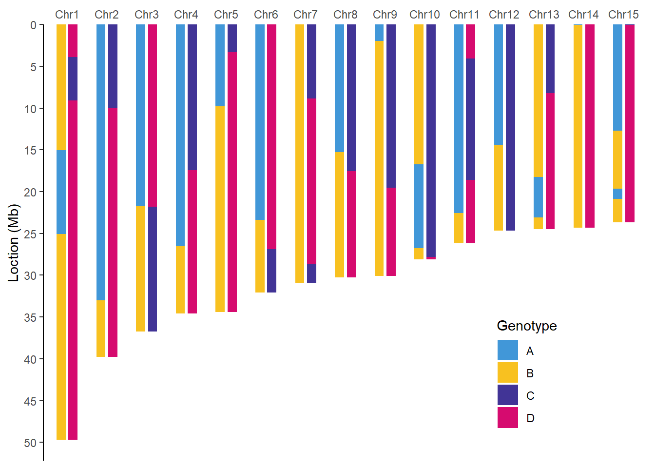
单家系全基因组基因型图
LepMap3输出默认的坐标和家系名称,根据实际坐标和名称对原始输出进行预处理
pos <- fs::dir_ls(path = str_c(path, "Lychee/Data/POS/"))

tmppos <- map_dfr(.x = pos,
                  .f = ~ read_tsv(., col_names = FALSE, show_col_types = FALSE),
                  .id = NULL) %>%
  `colnames<-`(c("chrom", "pos")) %>%
  group_by(chrom) %>%
  mutate(id = row_number(),
         markername = str_c(chrom, "-", id),
         marker = str_c(chrom, "_", pos)) %>%
  ungroup() %>%
  select(markername, marker)

file <- fs::dir_ls(path = str_c(path, "Lychee/Data/geno/"), glob = "*Ave*")

taxa <- read_tsv(file = str_c(path, "Lychee/extraMaterials/renametaxa.txt"),
                 show_col_types = FALSE,
                 col_names = FALSE)
tmp <- map_dfr(.x = file,
               .f = ~ read_tsv(., skip = 1, show_col_types = FALSE),
               .id = "Chrtmp") %>%
  rename_with(.cols = taxa$X2, ~ taxa$X1) %>%
  filter(MARKER != "MARKER") %>%
  mutate(chrom = sapply(str_split(str_replace(Chrtmp, path, ""), "/|_"), `[`, 4),
         markername = str_c(chrom, "-", MARKER),
         chr = str_sub(chrom, start = 4) %>% as.numeric(),
         pos = as.numeric(MALE_POS)) %>%
  select(markername, chr, pos, starts_with("F"), -FEMALE_POS) %>%
  mutate(across(.cols = starts_with("F"),
                ~ case_when(
                  . == "1 2" ~ "AD",
                  . == "1 1" ~ "AC",
                  . == "2 1" ~ "BC",
                  . == "2 2" ~ "BD"
                ))) %>%
  left_join(tmppos, by = "markername") %>%
  group_by(chr) %>%
  mutate(end = sapply(str_split(marker, "_"), `[`, 2) %>% as.numeric(),
         start = lag(end, default = 0)) %>%
  ungroup() %>%
  select(marker, chr, start, end, starts_with("F"))

head(tmp)
## # A tibble: 6 × 268
## marker chr start end F101 F10 F103 F104 F105 F107 F108 F109 F110
## <chr> <dbl> <dbl> <dbl> <chr> <chr> <chr> <chr> <chr> <chr> <chr> <chr> <chr>
## 1 Chr10… 10 0 2074 AD AD AD BD AD BD BD BD AC
## 2 Chr10… 10 2074 13977 AD AD AD BD AD BD BD BD AC
## 3 Chr10… 10 13977 32248 AD AD AD BD AD BD BD BD AC
## 4 Chr10… 10 32248 35953 AD AD AD BD AD BD BD BD AC
## 5 Chr10… 10 35953 53527 AD AD AD BD AD BD BD BD AC
## 6 Chr10… 10 53527 79901 AD AD AD BD AD BD BD BD AC
## # … with 255 more variables: F111 <chr>, F112 <chr>, F113 <chr>, F114 <chr>,
## # F115 <chr>, F116 <chr>, F118 <chr>, F119 <chr>, F1 <chr>, F120 <chr>,
## # F121 <chr>, F12 <chr>, F122 <chr>, F123 <chr>, F124 <chr>, F125 <chr>,
## # F126 <chr>, F127 <chr>, F128 <chr>, F129 <chr>, F131 <chr>, F13 <chr>,
## # F134 <chr>, F135 <chr>, F136 <chr>, F140 <chr>, F141 <chr>, F142 <chr>,
## # F143 <chr>, F144 <chr>, F145 <chr>, F146 <chr>, F147 <chr>, F148 <chr>,
## # F149 <chr>, F151 <chr>, F15 <chr>, F152 <chr>, F153 <chr>, F154 <chr>, …预处理文件第一列为标记,第二列染色体,第三四列为BIN的起始结束坐标,第五行后是家系基因型。
genome <- tmp %>%
  group_by(chr) %>%
  summarise(hapA = max(end),
            hapB = max(end)) %>%
  pivot_longer(cols = -chr,
               names_to = "Hap",
               values_to = "len")  #基础骨架
prefix <- tmp %>%
  select(-starts_with("F"))

names(tmp)[-c(1:3)] %>%
  map_dfc(~ tmp %>%
            select(all_of(.x)) %>%
            separate(col = .x,
                     into = str_c(.x, c("_hapA", "_hapB")),
                     sep = 1)) %>% #phasing haplotype
  bind_cols(prefix) %>%
  pivot_longer(cols = starts_with("F"),
               names_to = c("taxa", "Hap"),
               names_sep = "_",
               values_to = "geno") %>%
  filter(taxa %in% c("F1", "F2")) %>% #以F1和F2作为图示案例
  group_nest(taxa) %>%
  mutate(plot = map(data, ~ ggplot() +
                      geom_bar(data = genome,
                               mapping = aes(x = chr, y = len/1e6, group = Hap),
                               colour = "white",
                               stat = "identity",
                               fill = "white",
                               width = 0.4,
                               position = position_dodge2(width = 0.5)) +
                      scale_x_discrete(limits = str_c("Chr", seq(1, 15)),
                                       position = "top") +
                      scale_y_continuous(breaks = seq(0, 50, 5), # 酌情调整染色体数目和长度
                                         trans = "reverse",
                                         expand = expansion(mult = c(0.05, 0))) +
                      theme_bw() +
                      theme(legend.position = c(0.8, 0.2),
                            plot.background = element_blank() ,
                            panel.grid.major = element_blank(),
                            panel.grid.minor = element_blank() ,
                            panel.border = element_blank(),
                            axis.ticks.x = element_blank(),
                            axis.line.y = element_line()) +
                      xlab(NULL) + ylab("Loction (Mb)") +
                      geom_rect(data = .x,
                                mapping = aes(xmin = chr - 0.23,
                                              xmax = chr + 0.23,
                                              ymin = start/1e6,
                                              ymax = end/1e6,
                                              fill = geno,
                                              group = Hap),
                                position = position_dodge(width = 0.6)) +
                      scale_fill_manual(values = c( "#4197d8", "#f8c120", "#413496", "#d60b6f"),
                                        name = "Genotype"))) %>%
  walk2(.x = .$taxa,
        .y = .$plot,
        .f = ~ print(.y))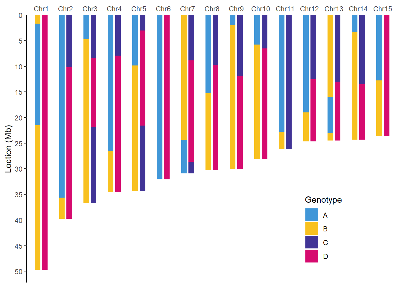
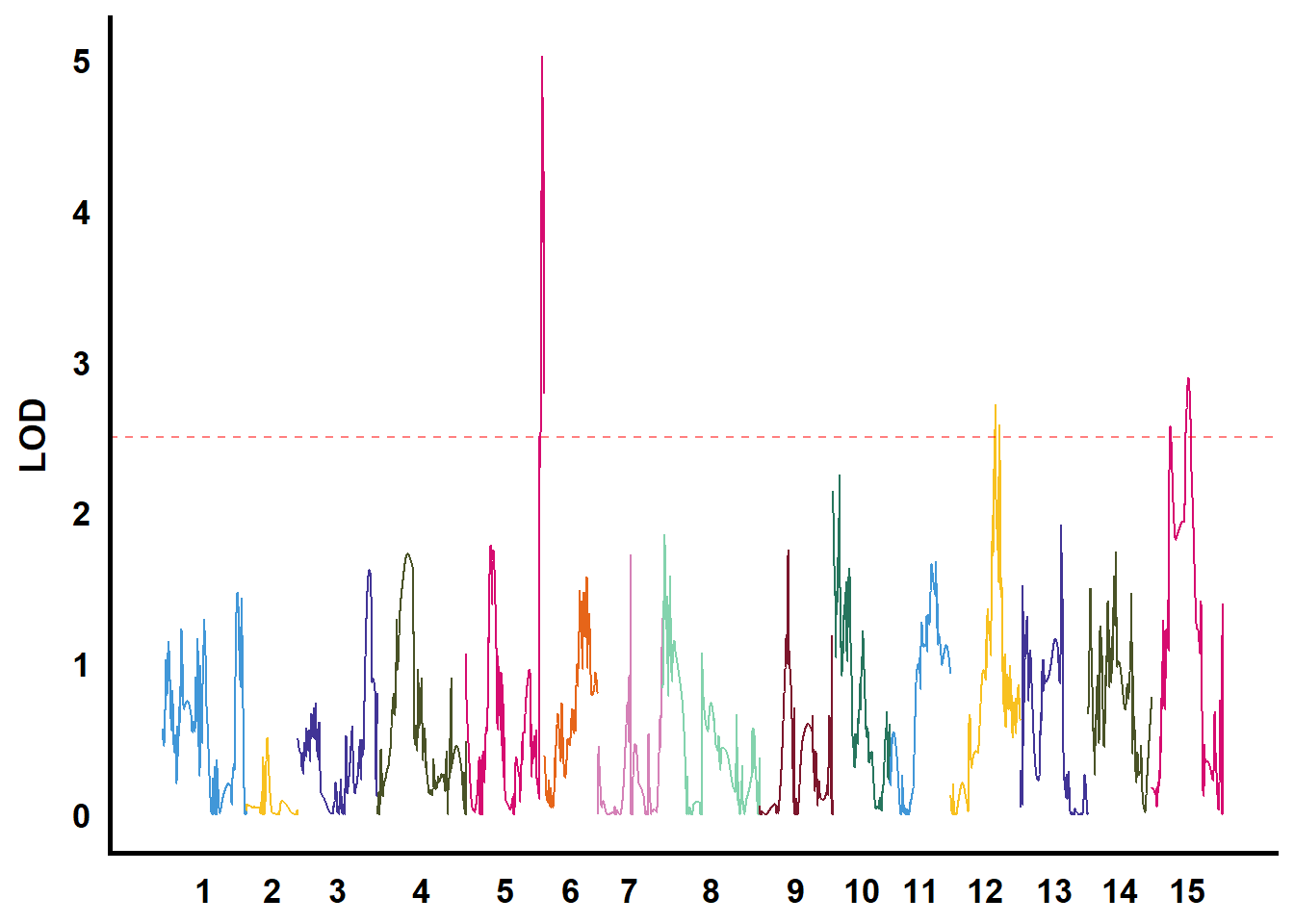
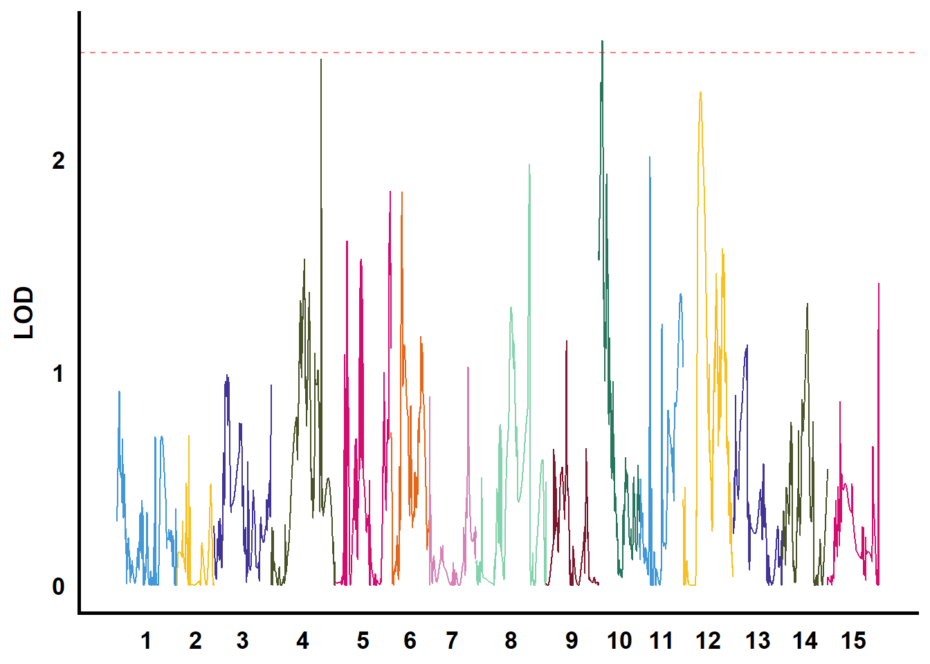
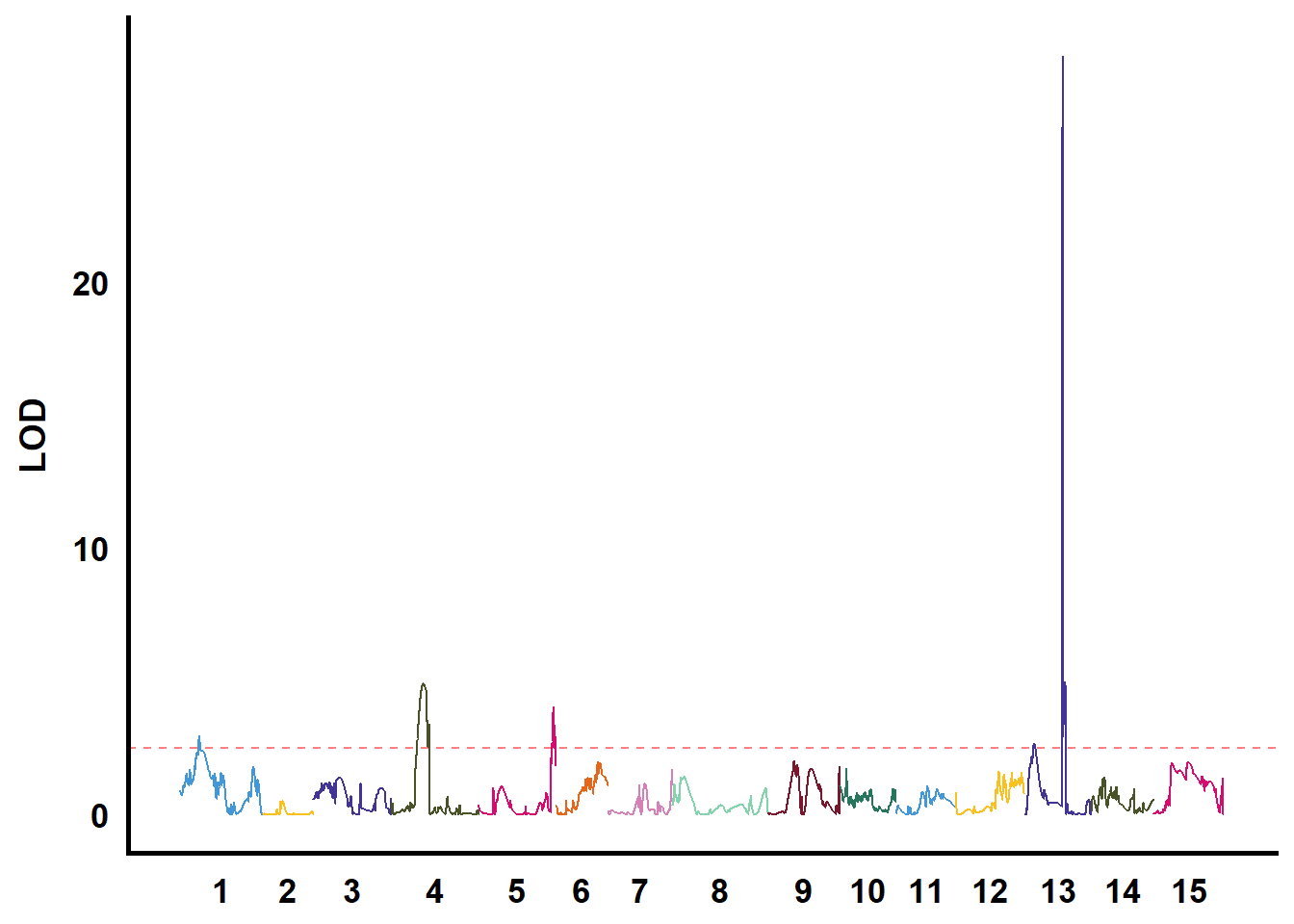
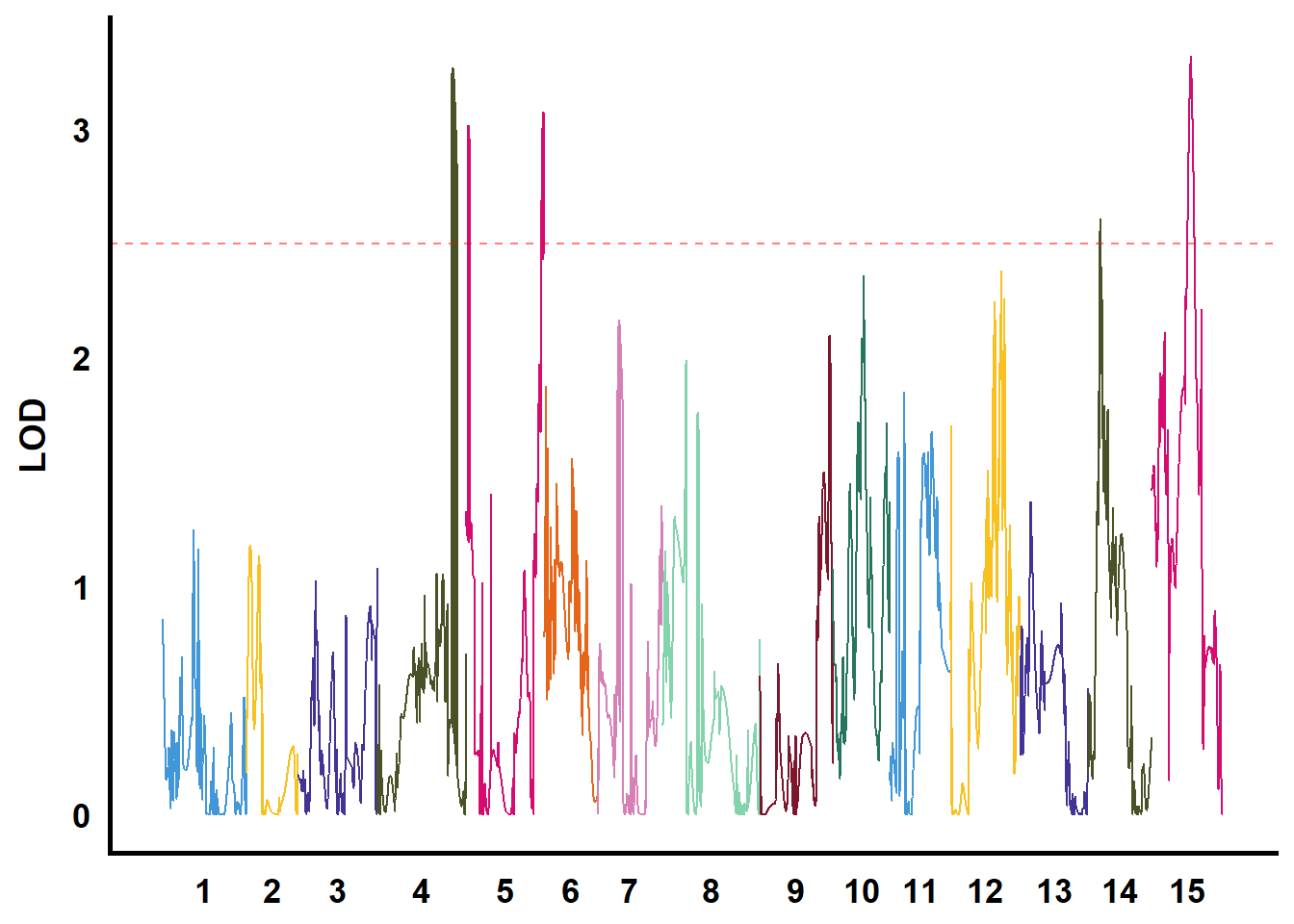
QTL作图
利用GACD软件进行连锁分析
path2 <- "C:/Users/wpf/Desktop/project/WinQTLMAP/GACD/Lychee/CDQ/LycheeGACD/Results/LycheeGACD.ric"

tmp <- fread(path2) %>%
  select(TraitName, Chromosome, Position, LOD) %>%
  group_by(TraitName) %>%
  mutate(pos = row_number()) %>%
  ungroup()

axis <- tmp %>%
  group_by(Chromosome) %>%
  summarise(center = mean(pos))

tmp %>%
  filter(str_starts(TraitName, pattern = "biyezhong")) %>%
  group_nest(TraitName) %>%
  mutate(plot = map(data, ~ ggplot() +
                      geom_line(data = .x,
                                mapping = aes(x = pos, y = LOD, colour = as.factor(Chromosome))) +
                      geom_hline(yintercept = 2.5,
                                 color = "red",
                                 linetype = "dashed",
                                 alpha = 0.5) +
                      scale_x_continuous(labels = axis$Chromosome,
                                         breaks = axis$center) +
                      scale_color_manual(values = rep(c("#4197d8", "#f8c120", "#413496", "#495226", "#d60b6f", "#e66519", "#d581b7", "#83d3ad", "#7c162c", "#26755d"), 12)) +
                      theme_prism() +
                      theme(legend.position = "none",
                            axis.ticks = element_blank()) +
                      xlab(NULL) +
                      ylab("LOD"))) %>%
  walk2(.x = .$TraitName,
        .y = .$plot,
        .f = ~ print(.y))