泛基因分析
基因是表型的基础。构建泛基因集是泛基因组分析的常见手段。
利用Orthofinder构建个体间的同源基因和非同源基因的集合,同源基因集合中所有个体中均出现的同源基因集即为core基因,在大于1个个体中出现的同源基因集为Dispensable基因,非同源基因集为Private基因,若基因组数目较多,可适当调整阈值添加soft-core基因。
同源基因鉴定
先试用bbmap修改基因组格式,使每行长度等于60,再利用agat保留最长的转录本,并转换为蛋白序列,最后利用Orthofinder鉴定同源基因集。
reformat.sh in=genome.fa out=genome_new.fa fastawrap=60
singularity exec -e ~/Singularity_lib/agat_0.8.sif agat_sp_keep_longest_isoform.pl -gff genome.gff3 -o genome_longest_isoform.gff3
singularity exec -e ~/Singularity_lib/agat_0.8.sif agat_sp_extract_sequences.pl -gff genome_longest_isoform.gff3 -f genome_new.fa -p -o genome.pep.fa
singularity exec -e ~/Singularity_lib/orthofinder_2.5.4.sif orthofinder -f 04.pep/ -t 20 -a 20
结果中的Orthogroups.tsv为同源基因集,Orthogroups_UnassignedGenes.tsv为非同源基因集。处理这两个数据集作为拟合泛基因集的输入。
group <- read_tsv("Genomics/Genetribe/data/Orthogroups.tsv", show_col_types = FALSE)
ungroup <-  read_tsv("Genomics/Genetribe/data/Orthogroups_UnassignedGenes.tsv", show_col_types = FALSE)

tmp <- group %>%
  bind_rows(ungroup) %>%
  mutate(ClusterID = row_number(),
         across(.col = -ClusterID,
                ~ if_else(is.na(.), "-", .))) %>%
  select(ClusterID, everything(), -Orthogroup)

write_tsv(tmp, "Genomics/Genetribe/output/founder_orthogroups.tsv")
利用PanGP图形界面软件构建泛基因集,输出Pandata及拟合函数以作图。
泛基因集拟合图
suppressWarnings(suppressMessages(library(tidyverse)))
suppressWarnings(suppressMessages(library(ggprism)))

pangenome <- function(x) {
  return(1.33087e7*(x**0.001)- 1.32709e7)
}
coregenome <- function(x) {
  return(31775.5 * exp(-0.64 * x) + 20916.1)
}

path <- "C:/Users/wpf/Desktop/project/Multiomics/"

tmp <- read_tsv(str_c(path, "Genomics/Genetribe/output/homologs/founder_pandata.tsv"), show_col_types = FALSE) %>%
  `colnames<-`(c("num", "pan", "core"))

pan <- tmp %>%
  select(num, pan) %>%
  filter(num != 8)

core <- tmp %>%
  select(num, core) %>%
  filter(num != 1 & num != 8)

curve <- tibble(
  num = seq(1, 8, 0.1),
  pan = pangenome(num),
  core = coregenome(num)
) %>%
  pivot_longer(cols = -num)

ggplot() +
  geom_boxplot(data = pan,
               mapping = aes(x = num,
                             y = pan,
                             group = num),
               width = 0.6,
               color = "#8F2D56") +
  geom_boxplot(data = core,
               mapping = aes(x = num,
                             y = core,
                             group = num),
               width = 0.6,
               color = "#6AAFE6") +
  geom_line(data = curve,
            mapping = aes(x = num,
                          y = value,
                          colour = name)) +
  scale_colour_manual(limits = c("pan", "core"),
                      values = c("#8F2D56", "#6AAFE6"),
                      labels = c("Pan-Gene", "Core-Gene")) +
  theme_prism() +
  theme(legend.position = c(0.8, 0.5)) +
  labs(x = "Genome Number", y = "Gene Cluster Number (K)")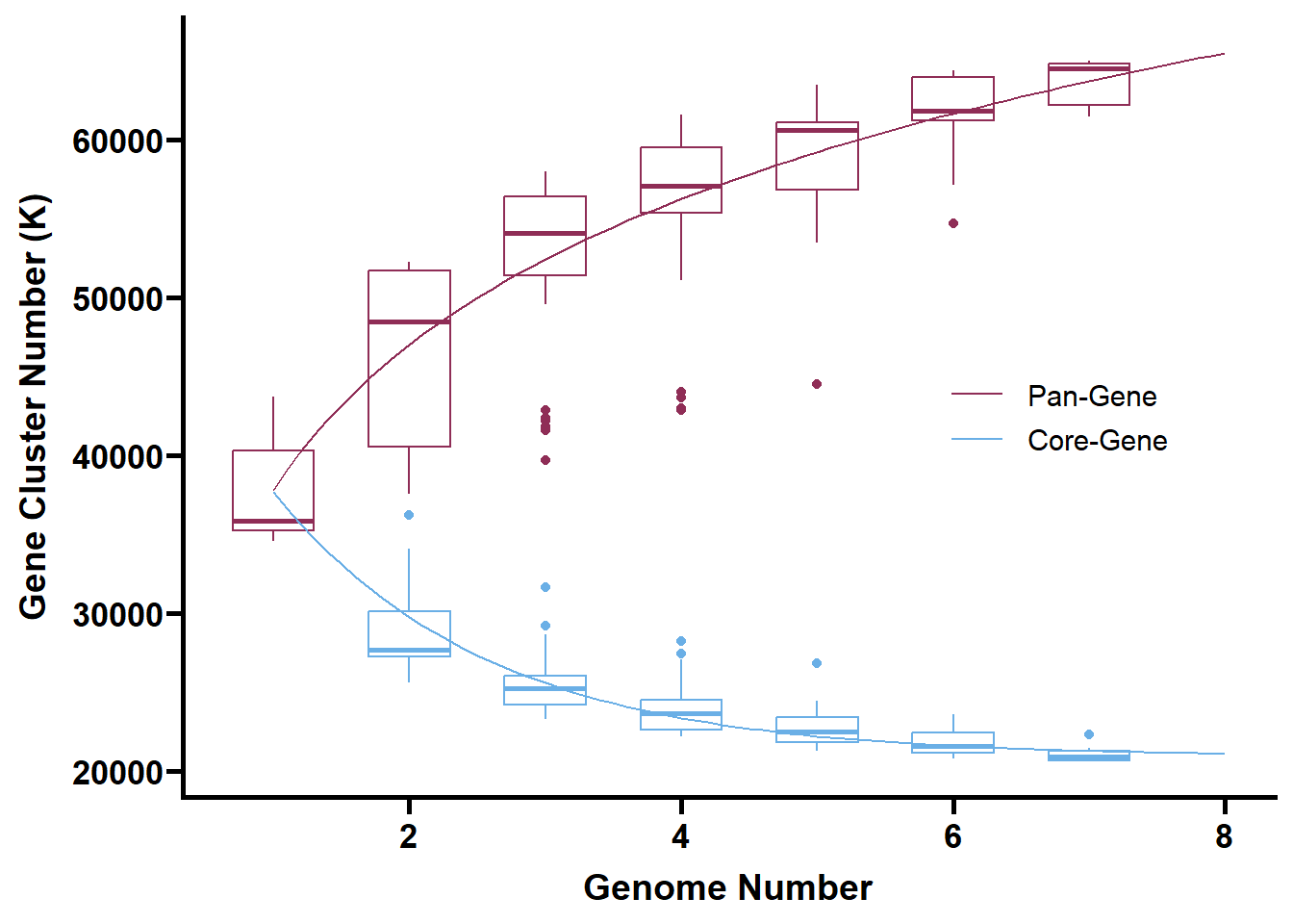
泛基因集饼图
tmp <- read_tsv(str_c(path, "Genomics/Genetribe/output/homologs/founder_orthogroups.tsv"), show_col_types = FALSE) %>%
  mutate(across(.col = -ClusterID,
                ~ if_else(. == "-", NA_character_, .))) %>%
  mutate(n = rowSums(is.na(.)),
         type = case_when(
           n == 0 ~ "Core",
           n == 7 ~ "Private",
           TRUE ~ "Dispensable"
         ))

tmp2 <- tmp %>%
  count(type) %>%
  arrange(desc(type)) %>%
  mutate(rate = 100*n/sum(n),
         lab = cumsum(rate) - rate/2)

ggplot(data = tmp2) +
  geom_bar(mapping = aes(x = 2,
                         y = rate,
                         fill = type),
           stat = "identity",
           color = "white") +
  coord_polar(theta = "y",
              start = 0) +
  geom_text(mapping = aes(x = 2,
                          y = lab,
                          label = signif(rate, digits = 4)),
            color = "white") +
  scale_fill_manual(values = c("#6AAFE6", "#F6B352", "#5c196b")) +
  theme_void() +
  theme(legend.position = "none") +
  xlim(0.5, 2.5)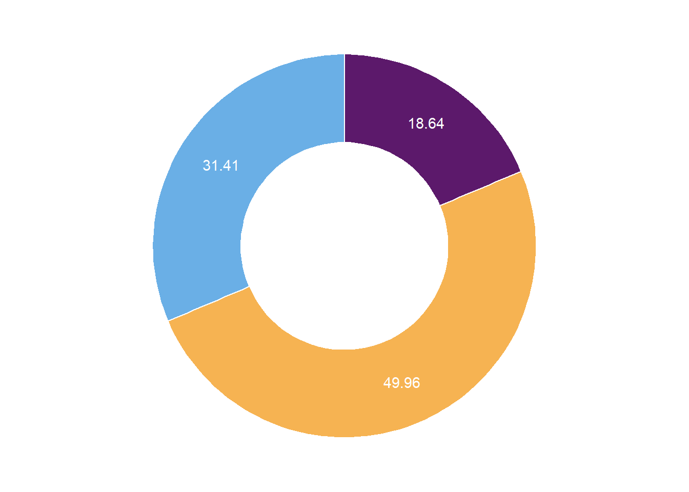
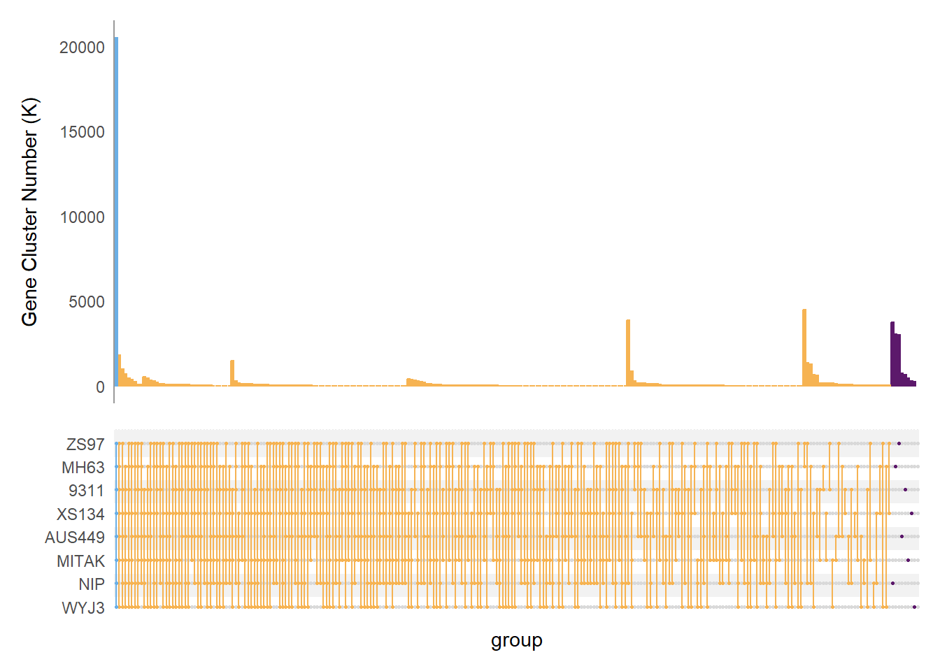
泛基因集upset图
suppressWarnings(suppressMessages(library(ComplexUpset)))

tmp2 <- tmp %>%
  mutate(across(.col = -c(n, type, ClusterID),
                ~ case_when(
                  is.na(.) ~ 0,
                  TRUE ~ 1
                ))) %>%
  rename(NIP = nip,
         MITAK = Mitak)

name <- rev(c("ZS97", "MH63", "9311", "XS134", "AUS449", "MITAK", "NIP", "WYJ3"))

query_by_degree = function(data, groups, params_by_degree, ...) {
  intersections = unique(upset_data(data, groups)$plot_intersections_subset)
  lapply(
    intersections,
    FUN = function(x) {
      members = str_split_1(x, "-")
      if (!(length(members) %in% names(params_by_degree))) {
        stop(
          paste('Missing specification of params for degree', length(members))
        )
      }
      args = c(
        list(intersect = members, ...),
        params_by_degree[[length(members)]]
      )
      do.call(upset_query, args)
    }
  )
}

upset(data = tmp2,
      intersect = name,
      matrix = intersection_matrix(
        geom = geom_point(size = 0.5)
      ),
      width_ratio = 0.1,
      intersections = "all",
      sort_intersections_by = c("degree", "cardinality"),
      sort_set = FALSE,
      set_sizes = FALSE,
      base_annotations = list(
        "Gene Cluster Number (K)" = intersection_size(
          counts = FALSE
      ) + theme(panel.grid = element_blank(),
                axis.line.y = element_line(colour = "grey60"))),
      queries = query_by_degree(
        tmp2,
        name,
        params_by_degree = list(
          "1" = list(fill = "#5c196b", color = "#5c196b"),
          "2" = list(fill = "#F6B352", color = "#F6B352"),
          "3" = list(fill = "#F6B352", color = "#F6B352"),
          "4" = list(fill = "#F6B352", color = "#F6B352"),
          "5" = list(fill = "#F6B352", color = "#F6B352"),
          "6" = list(fill = "#F6B352", color = "#F6B352"),
          "7" = list(fill = "#F6B352", color = "#F6B352"),
          "8" = list(fill = "#6AAFE6", color = "#6AAFE6")
        ),
        only_components=c("intersections_matrix", "Gene Cluster Number (K)")
      ))
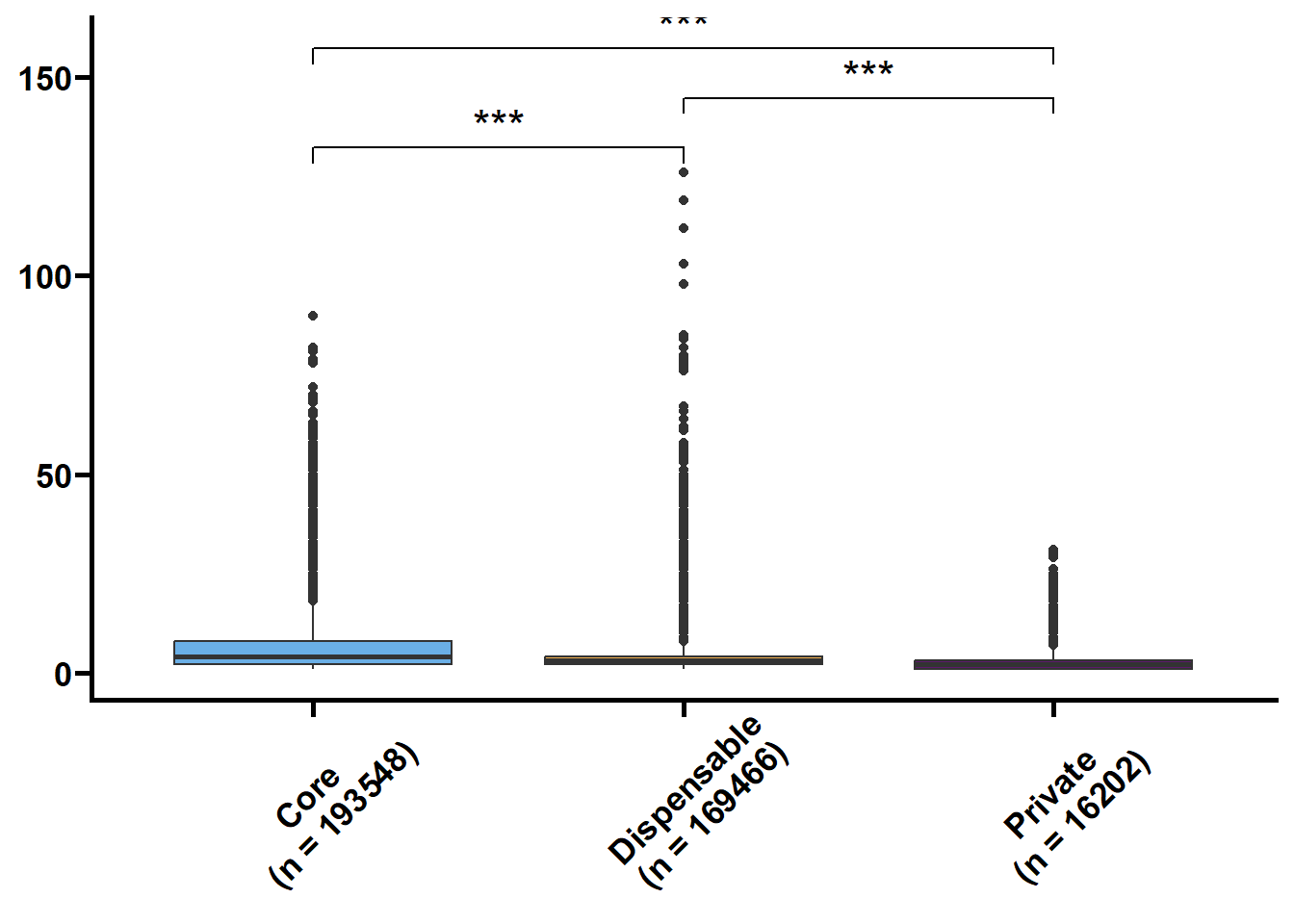
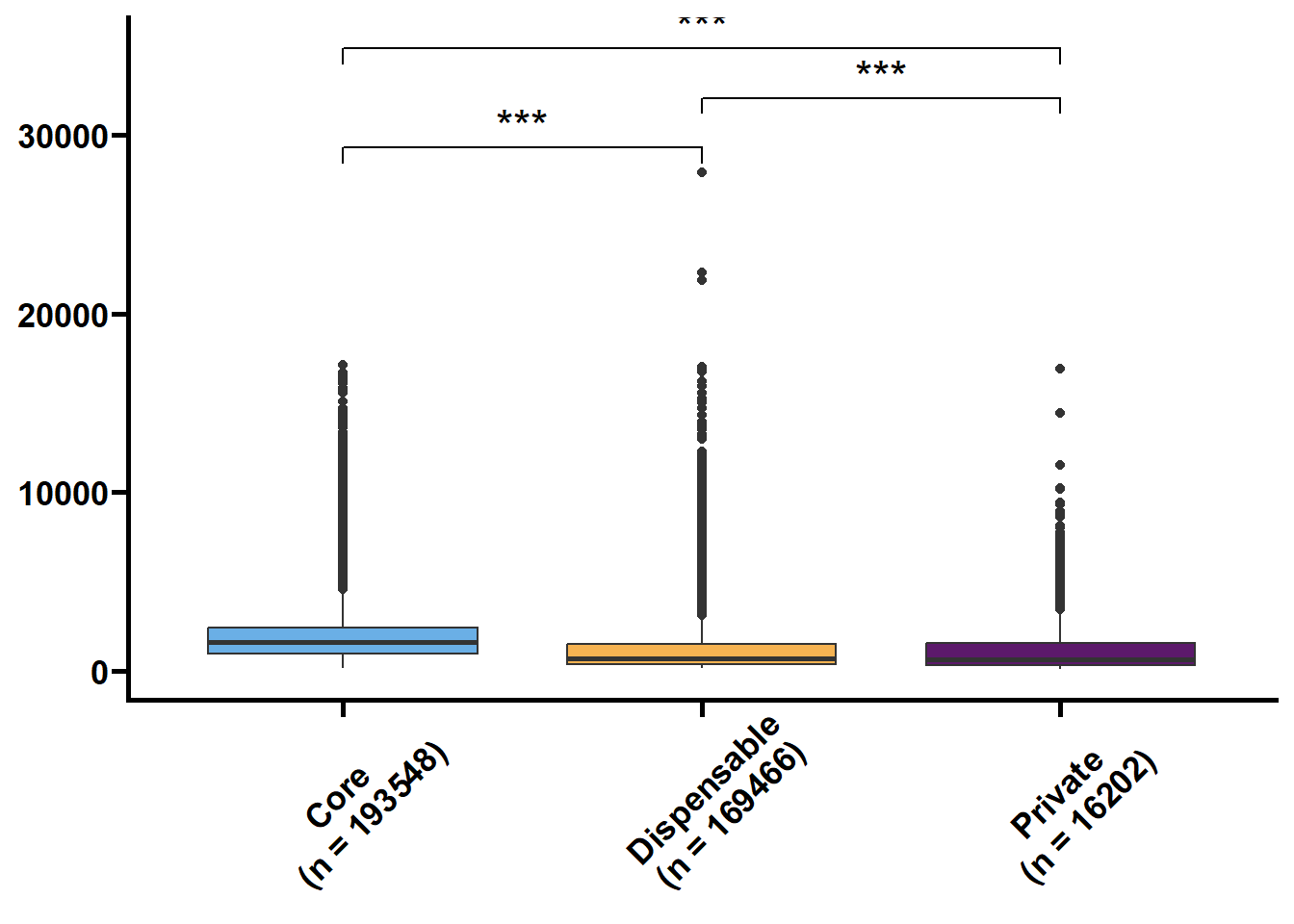
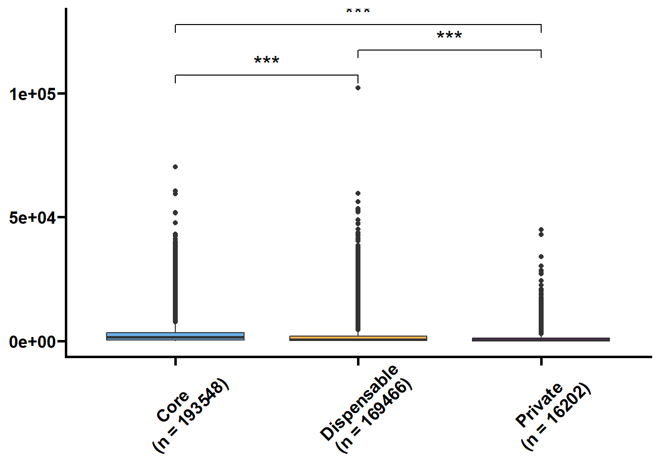
泛基因集特征统计
基因组统计
基因长度,外显子和内含子的长度和个数是基因的基本特征,我们想看看在核心基因和非核心间这些特征是否存在差异。可变剪接也是重要的特征,但我们的注释缺乏转录组的支撑,故可变剪接的注释准确性不高。
利用agat根据gff提取基因特征
singularity exec -e ~/Singularity_lib/agat_0.8.sif agat_convert_sp_gff2bed.pl --gff genome.gff -o genome.bedsuppressWarnings(suppressMessages(library(ggsignif)))
suppressWarnings(suppressMessages(library(data.table)))
bedfile <- fs::dir_ls(str_c(path, "Genomics/Genetribe/data/Bed/founder/"))
bed <- map_dfr(.x = bedfile,
.f = ~ fread(.),
.id = "id") %>%
mutate(taxa = str_replace(id, pattern = ".*/", "") %>% str_sub(end = -5),
gene = str_split_i(V4, "[\\.-]", 1),
genelength = V8 - V7,
exon = V10,
intron = exon - 1) %>%
rowwise() %>%
mutate(exonlength = sum(as.numeric(str_split_1(V11, ","))),
intronlength = as.numeric(str_split_i(V12, ",", exon)) - exonlength + as.numeric(str_split_i(V11, ",", exon))) %>%
select(taxa, gene, genelength, exon, intron, exonlength, intronlength)
tmp2 <- tmp %>%
select(-c(ClusterID, n)) %>%
pivot_longer(cols = -type,
names_to = "taxa",
values_to = "gene") %>%
separate_longer_delim(cols = gene, delim = ", ") %>%
drop_na() %>%
mutate(gene = str_split_i(gene, "\\.", 1)) %>%
left_join(bed, by = c("taxa", "gene")) %>%
pivot_longer(cols = -c(type, taxa, gene),
names_to = "group")
tmp2 %>%
nest(.by = group) %>%
mutate(plot = map(.x = data,
.f = ~ ggplot(data = .x,
mapping = aes(x = type,
y = value,
fill = type)) +
geom_boxplot() +
geom_signif(
comparisons = list(c("Core", "Dispensable"), c("Dispensable", "Private"), c("Core", "Private")),
map_signif_level = TRUE,
textsize = 6,
step_increase = 0.1
) +
scale_fill_manual(values = c("#6AAFE6", "#F6B352", "#5c196b")) +
scale_x_discrete(limits = c("Core", "Dispensable", "Private"),
labels = c("Core\n(n = 193548)", "Dispensable\n(n = 169466)", "Private\n(n = 16202)")) +
theme_prism() +
theme(legend.position = "none",
axis.text.x = element_text(angle = 45, hjust = 0.4)) +
labs(x = NULL, y = NULL))) %>%
walk2(.x = .$group,
.y = .$plot,
.f = ~ print(.y))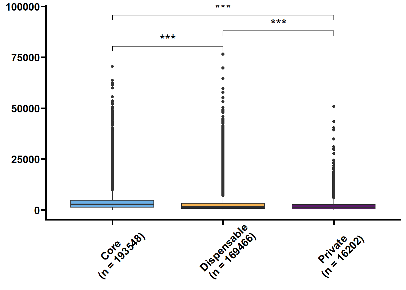

群体遗传统计
Ka/Ks表示非同义替换位点替换次数(Ka)与同义替换位点替换次数(Ks)的比值,这个比例可用于判断这个基因是否存在选择压力。
一把来说,Ka >> Ks或者Ka/Ks >> 1,基因受正选择(positive selection);Ka=Ks或者Ka/Ks = 1,基因中性进化(neutral evolution);Ka << Ks或者Ka/Ks << 1,基因受纯化选择(purify selection)。
先将Orthofinder的同源基因集按core和dispensable分类
tmp %>%
  select(-n) %>%
  pivot_longer(cols = -c(ClusterID, type),
               names_to = "taxa",
               values_to = "gene") %>%
  separate_longer_delim(cols = gene, delim = ", ") %>%
  drop_na() %>%
  mutate(gene = str_split_i(gene, "\\.", 1)) %>%
  group_by(ClusterID) %>%
  summarise(homologs = str_c(gene, collapse = "\t")) %>%
  left_join(tmp, by = "ClusterID") %>%
  select(type, homologs) %>%
  nest(.by = type) %>%
  walk2(.x = .$type,
        .y = .$data,
        .f = ~ write_tsv(.y, file = str_c("Genomics/Genetribe/output/homologs/", .x, "homologs.tsv"), col_names = FALSE))

tmp %>%
  select(-n) %>%
  pivot_longer(cols = -c(ClusterID, type),
               names_to = "taxa",
               values_to = "gene") %>%
  separate_longer_delim(cols = gene, delim = ", ") %>%
  drop_na() %>%
  mutate(gene = str_split_i(gene, "\\.", 1)) %>%
  select(type, gene) %>%
  nest(.by = type) %>%
  walk2(.x = .$type,
        .y = .$data,
        .f = ~ write_tsv(.y, file = str_c("Genomics/Genetribe/output/homologs/", .x, "gene.tsv"), col_names = FALSE))
准备输入文件,先提取最长转录本的cds序列,再转换为蛋白质序列,最后根据基因ID分类
利用ParaAT.pl和KaKs_Calculator计算每个同源基因集的Ka/Ks, 部分同源基因集会出现多重比对的长度不等的情况,超出解决范围,只能留待将来再用到的时候考虑另一个工具或另一种同源基因数据集。
module load ClustalW2/2.1

ParaAT.pl -h Dispensablehomologs.tsv -a ../03.groupfasta/dispensable.pep.fa -n ../03.groupfasta/dispensable.cds.fa -p proc -m clustalw2 -f axt -o dispensableaxt

KaKs -i dispensableaxt/ClusterID1.cds_aln.axt -O ClusterID1.kaks
合并kaks
file <- fs::dir_ls(path = "Genomics/Genetribe/data/KaKs/", type = "file", recurse = TRUE)

Kaks <- map_dfr(.x = file,
                .f = ~ read_tsv(., show_col_types = FALSE),
                .id = "file")

write_tsv(Kaks, file = "Genomics/Genetribe/output/homologs/KaKs.tsv")
Kaks <- read_tsv(str_c(path, "Genomics/Genetribe/output/homologs/KaKs.tsv"), show_col_types = FALSE) %>%
mutate(type = str_split_i(file, "/", 5) %>% str_replace("KaKs", "")) %>%
select(type, Ka, Ks, `Ka/Ks`) %>%
drop_na() %>%
rename(Ka_Ks = `Ka/Ks`) %>%
pivot_longer(cols = -type,
names_to = "group")
Kaks %>%
filter(value <= 2) %>%
nest(.by = group) %>%
mutate(plot = map(.x = data,
.f = ~ ggplot(data = .x,
mapping = aes(x = type,
y = value,
fill = type)) +
geom_boxplot() +
geom_signif(
comparisons = list(c("core", "dispensable")),
map_signif_level = TRUE,
textsize = 6,
step_increase = 0.1
) +
scale_fill_manual(values = c("#6AAFE6", "#F6B352")) +
scale_x_discrete(limits = c("core", "dispensable"),
labels = c("Core", "Dispensable")) +
theme_prism() +
theme(legend.position = "none",
axis.text.x = element_text(angle = 45, hjust = 0.4)) +
labs(x = NULL, y = NULL))) %>%
walk2(.x = .$group,
.y = .$plot,
.f = ~ print(.y))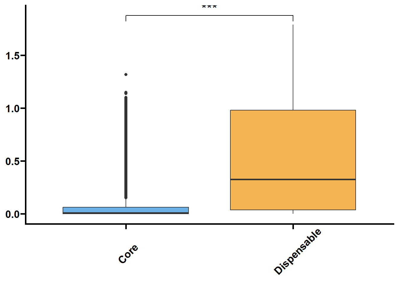
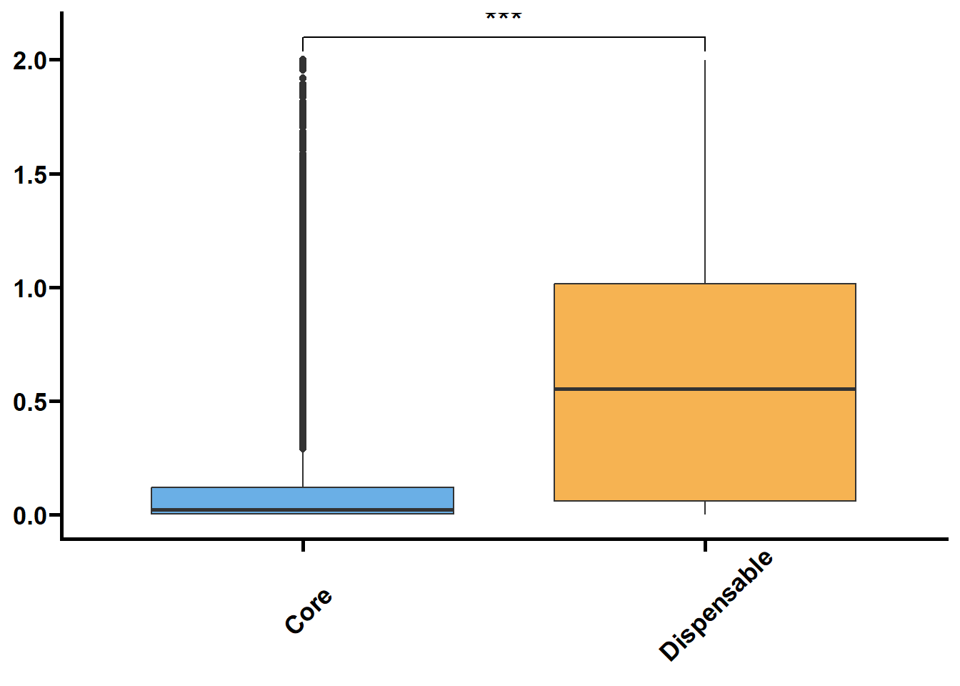
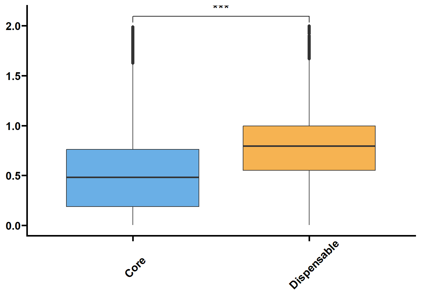
核苷酸多样度(θπ和Watterson θw)反映了群体内不同个体DNA序列间的观察平均碱基差异占比,被广泛用于表征种群的遗传多样度水平。Tajima’s D是由日本研究员田田文雄(Fumio Tajima)创建的群体基因检验统计数据,可以用于区分DNA序列是随机进化还是受到自然选择。
利用533群体的SNP数据来鉴定核心基因和非核心基因的群体遗传参数。
以前利用vcftools可以直接计算窗口内的pi和TajimaD,对于以基因为窗口则使用python包tajimas-d。核心思路是先提取各个基因的VCF,再利用seqkit和bcftools生成各个样本的序列,再利用tajimas-d计算θπ,θw和tajimaD值,其中θπ和θw需除以各自基因的全长。
nip <- read_tsv("Genomics/Genetribe/data/Bed/founder/nip.bed", show_col_types = FALSE, col_names = FALSE) %>%
  mutate(chrom = str_c("Chr", as.numeric(str_sub(X1, start = 4))),
         gene = str_split_i(X4, "\\.", 1)) %>%
  select(chrom, X2, X3, gene)

write_tsv(nip, file = "Genomics/Genetribe/output/founder/nip.bed", col_names = FALSE)
cat nip.bed |while read i j k l;do bcftools filter 533.vcf.gz -r ${i}:${j}-${k} -Oz -o ${l}.vcf.gz;bcftools index ${l}.vcf.gz;seqkit faidx genome.fa ${i}:${j}-${k} > ${l}.fa;done
cat gene.list|while read i;do mkdir ${i}fasta; cat sample.list|while read j;do bcftools consensus -f ${i}.fa ${i}.vcf.gz -s ${j} -p ${j} > ${i}fasta/${j}.fa;done;cat ${i}fasta/*.fa > ../VCF2fasta/${i}.fa;rm -rf ${i}fasta/;done
cat gene.list|while read i;do bsub -J ${i} -n 1 -q short "singularity exec -e ~/Singularity_lib/tajimas_d.sif tajimas_d -f ../VCF2fasta/${i}.fa -p > pi/${i}.pi;singularity exec -e ~/Singularity_lib/tajimas_d.sif tajimas_d -f ../VCF2fasta/${i}.fa -w > watterson/${i}.watterson;singularity exec -e ~/Singularity_lib/tajimas_d.sif tajimas_d -f ../VCF2fasta/${i}.fa -t > tajima/${i}.tajima";done
grep "" pi/*pi > nipgene.pi
grep "" tajima/*tajima > nipgene.tajima
grep "" watterson/*watterson > nipgene.wattersonnipbed <- read_tsv(str_c(path, "Genomics/Genetribe/output/founder/nip.bed"), col_names = FALSE, show_col_types = FALSE) %>%
`colnames<-`(c("chrom", "start", "end", "gene"))
pi <- read_tsv(str_c(path, "Genomics/Genetribe/data/PI/nipgene.pi"), show_col_types = FALSE, col_names = FALSE) %>%
mutate(gene = str_split_i(X1, "[/.]", 2)) %>%
rename(pi = X3) %>%
select(gene, pi) %>%
filter(pi != 0)
watterson <- read_tsv(str_c(path, "Genomics/Genetribe/data/PI/nipgene.watterson"), show_col_types = FALSE, col_names = FALSE) %>%
mutate(gene = str_split_i(X1, "[/.]", 2)) %>%
rename(watterson = X2) %>%
select(gene, watterson) %>%
filter(watterson != 0)
tajima <- read_tsv(str_c(path, "Genomics/Genetribe/data/PI/nipgene.tajima"), show_col_types = FALSE, col_names = FALSE) %>%
mutate(gene = str_split_i(X1, "[/.]", 2)) %>%
rename(tajima = X3) %>%
select(gene, tajima) %>%
filter(tajima != 0)
tmp2 <- tmp %>%
select(-c(ClusterID, n)) %>%
pivot_longer(cols = -type,
names_to = "taxa",
values_to = "gene") %>%
separate_longer_delim(cols = gene, delim = ", ") %>%
drop_na() %>%
filter(taxa == "nip") %>%
mutate(gene = str_split_i(gene, "\\.", 1)) %>%
left_join(nipbed, by = "gene") %>%
left_join(pi, by = "gene") %>%
left_join(watterson, by = "gene") %>%
left_join(tajima, by = "gene") %>%
mutate(len = end - start,
pi = pi/len,
watterson = watterson/len) %>%
select(type, pi, watterson, tajima) %>%
pivot_longer(cols = -type)
tmp2 %>%
nest(.by = name) %>%
mutate(plot = map(.x = data,
.f = ~ ggplot(data = .x,
mapping = aes(x = type,
y = value,
fill = type)) +
geom_boxplot() +
geom_signif(
comparisons = list(c("Core", "Dispensable"), c("Dispensable", "Private"), c("Core", "Private")),
map_signif_level = TRUE,
textsize = 6,
step_increase = 0.1
) +
scale_fill_manual(values = c("#6AAFE6", "#F6B352", "#5c196b")) +
scale_x_discrete(limits = c("Core", "Dispensable", "Private"),
labels = c("Core\n(n = 19809)", "Dispensable\n(n = 12455)", "Private\n(n = 2234)")) +
theme_prism() +
theme(legend.position = "none",
axis.text.x = element_text(angle = 45, hjust = 0.4)) +
labs(x = NULL, y = NULL))) %>%
walk2(.x = .$name,
.y = .$plot,
.f = ~ print(.y))## Warning: Removed 21290 rows containing non-finite values (`stat_boxplot()`).## Warning: Removed 21290 rows containing non-finite values (`stat_signif()`).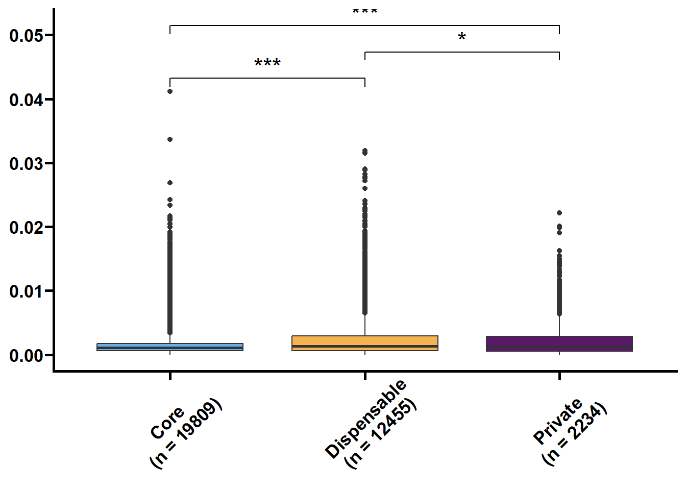
## Warning: Removed 21282 rows containing non-finite values (`stat_boxplot()`).## Warning: Removed 21282 rows containing non-finite values (`stat_signif()`).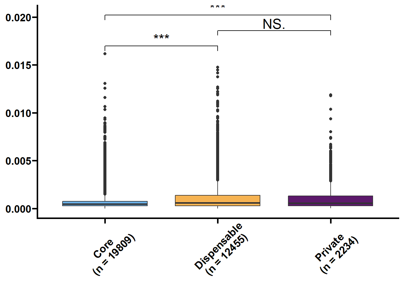
## Warning: Removed 21301 rows containing non-finite values (`stat_boxplot()`).## Warning: Removed 21301 rows containing non-finite values (`stat_signif()`).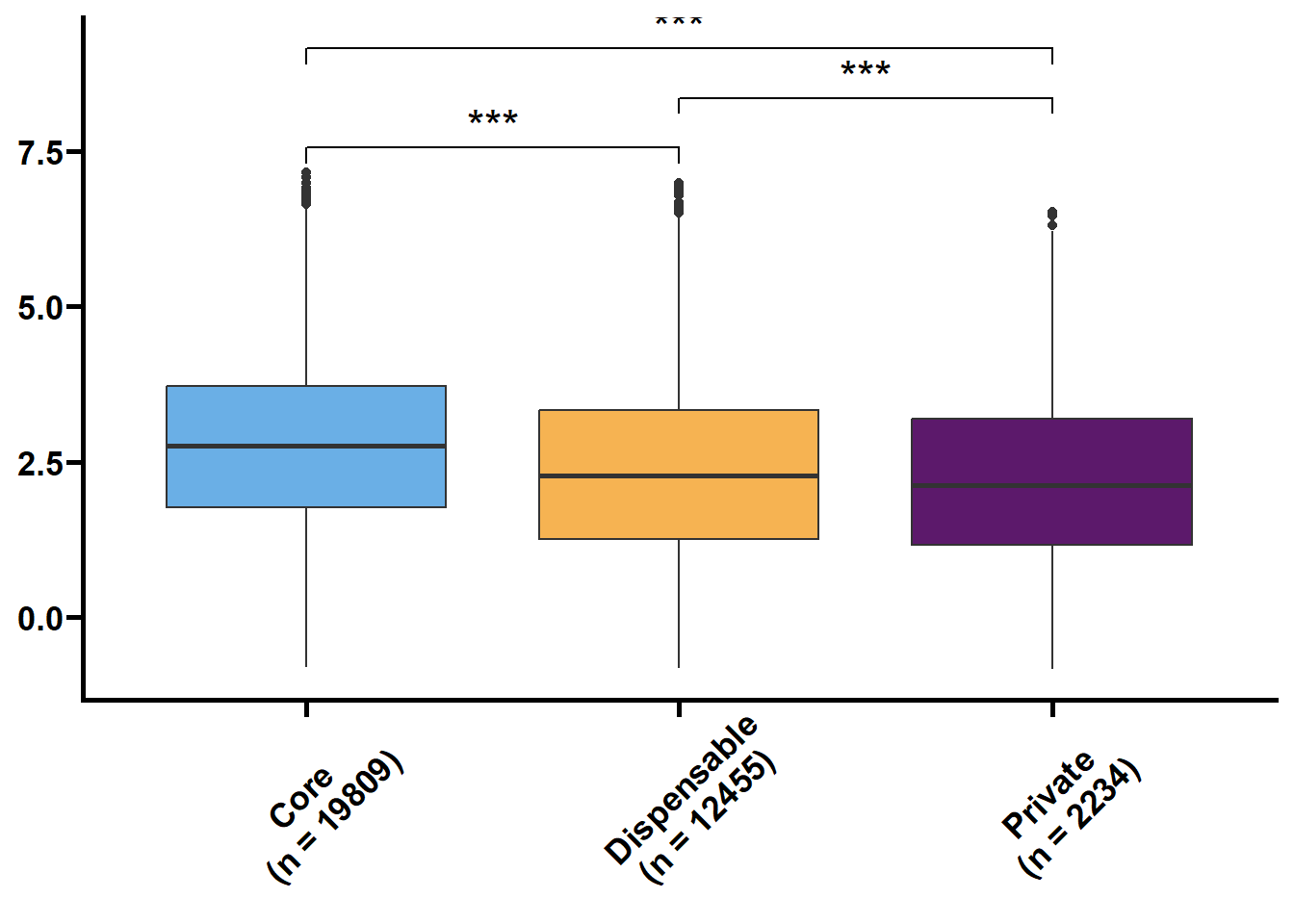 ##### 转录水平统计
利用明恢63四个组织的转录组定量来探究核心基因和非核心基因的转录水平关系。
# HISAT2 + Stringtie(stringtie会出现单个基因ID对应多个转录本TPM的现象,目前我的解决方式是直接相加)
i=$1

fastp -i ../01.Raw_seq/${i}_1.fq.gz -o ../02.paired/${i}_1.paired.fq.gz -I ../01.Raw_seq/${i}_2.fq.gz -O ../02.paired/${i}_2.paired.fq.gz -j ../02.paired/${i}.json -h ../02.paired/${i}.html -c -w 2 > ../00.log/fastp/${i}.log 2>&1

singularity exec -e ~/Singularity_lib/RNAseq.sif hisat2 -p 8 -x /public/home/pfwang/wpf/Datasets/Reference/Rice/NIP_MSU/HISAT2/nip -1 ../02.paired/${i}_1.paired.fq.gz -2 ../02.paired/${i}_2.paired.fq.gz -S ../03.Bam/${i}.sam > ../00.log/hisat2/${i}.log 2>&1

singularity exec -e ~/Singularity_lib/RNAseq.sif samtools view -@ 8 -b ../03.Bam/${i}.sam| singularity exec -e ~/Singularity_lib/RNAseq.sif samtools sort -@ 8 -o ../03.Bam/${i}.sort.bam
singularity exec -e ~/Singularity_lib/RNAseq.sif samtools index ../03.Bam/${i}.sort.bam
rm ../03.Bam/${i}.sam

mkdir -p ../04.Count/${i}
singularity exec -e ~/Singularity_lib/RNAseq.sif stringtie -B -e -p 8 -G ~/wpf/Datasets/Reference/Rice/NIP_MSU/nip.gff3 -o ../04.Count/${i}/transcripts.gtf -A ../04.Count/${i}/gene_abundances.tsv ../03.Bam/${i}.sort.bam
利用R语言合并多个样本的表达量文件
file <- fs::dir_ls(path = "RNAseq/ZSMH/data/", type = "file", recurse = TRUE)

tmptpm <- map_dfr(.x = file,
               .f = ~ read_tsv(., show_col_types = FALSE) %>%
                 select(`Gene ID`, TPM),
               .id = "file") %>%
  rename(gene = `Gene ID`) %>%
  mutate(taxa = str_split_i(file, "/", 4)) %>%
  group_by(gene, taxa) %>%
  summarise(TPM = sum(TPM)) %>%
  pivot_wider(id_cols = gene,
              names_from = taxa,
              values_from = TPM)

write_tsv(tmptpm, file = "RNAseq/ZSMH/output/TPM.tsv")
TPM <- read_tsv(str_c(path, "RNAseq/ZSMH/output/TPM.tsv"), show_col_types = FALSE) %>%
select(gene, starts_with("flagleaf_MH63_HTLD"), starts_with("panicle_MH63_HTLD"),
starts_with("root_MH63_HTLD"), starts_with("shoot_MH63_HTLD")) %>%
pivot_longer(cols = -gene,
names_sep = "_MH63_HTLD_",
names_to = c("issue", "rep")) %>%
group_by(gene, issue) %>%
summarise(value = sum(value))## `summarise()` has grouped output by 'gene'. You can override using the
## `.groups` argument.tmp2 <- tmp %>%
select(-c(ClusterID, n)) %>%
pivot_longer(cols = -type,
names_to = "taxa",
values_to = "gene") %>%
separate_longer_delim(cols = gene, delim = ", ") %>%
drop_na() %>%
mutate(gene = str_split_i(gene, "\\.", 1)) %>%
filter(taxa == "nip") %>%
left_join(TPM, by = "gene", multiple = "all") %>%
group_by(gene) %>%
filter(any(value > 0))
tmp2 %>%
ungroup() %>%
nest(.by = issue) %>%
mutate(plot = map(.x = data,
.f = ~ ggplot(data = .x,
mapping = aes(x = type,
y = log(value + 1),
fill = type)) +
geom_boxplot() +
geom_signif(
comparisons = list(c("Core", "Dispensable"), c("Dispensable", "Private"), c("Core", "Private")),
map_signif_level = TRUE,
textsize = 6,
step_increase = 0.1
) +
scale_fill_manual(values = c("#6AAFE6", "#F6B352", "#5c196b")) +
scale_x_discrete(limits = c("Core", "Dispensable", "Private"),
labels = c("Core\n(n = 22197)", "Dispensable\n(n = 12972)", "Private\n(n = 2495)")) +
theme_prism() +
theme(legend.position = "none",
axis.text.x = element_text(angle = 45, hjust = 0.4)) +
labs(x = NULL, y = NULL))) %>%
walk2(.x = .$issue,
.y = .$plot,
.f = ~ print(.y))![]()
![]()
![]()
![]()
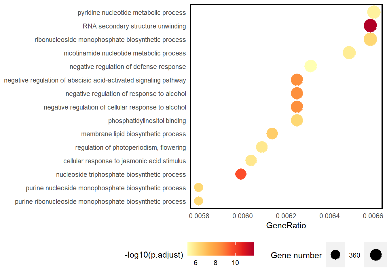
富集分析
基因富集分析,是分析基因表达信息的一种方法。富集是将基因按照先验知识,即基因组注释信息,对基因进行分类的过程,能够帮助寻找到的基因是否存在共性。
我们利用eggNOG-Mapper注释基因,再使用R包clusterProfiler进行富集分析。
# 准备比对数据库文件,解压使用
wget -c http://eggnog6.embl.de/download/emapperdb-5.0.2/eggnog.db.gz
wget -c http://eggnog6.embl.de/download/emapperdb-5.0.2/eggnog_proteins.dmnd.gz

singularity exec -e ~/Singularity_lib/agat_0.8.sif agat_sp_extract_sequences.pl -g ../00.gff/${i}_longest_isoform.gff -f ../00.gff/${i}_reformat.fa -t cds -o ${i}.cds
singularity exec -e ~/Singularity_lib/eggnog-mapper.sif emapper.py -i ../01.cds/${i}.cds --itype CDS -m diamond --data_dir ~/wpf/Datasets/Eggnog/ -o ${i} --cpu 20
准备GO注释文件,使用python代码get_go_term.py
#get_go_term.py
import sys
raw_file = open(sys.argv[1]).read()
with open("go_term.list","w") as output:
     for go_term in raw_file.split("[Term]"):
         go_id = ''
         name = ''
         namespace = ''
         for line in go_term.split("\n"):
             if str(line).startswith("id") and "GO:" in line:
                 go_id = line.rstrip().split(" ")[1]
             if str(line).startswith("name:"):
                 name = line.rstrip().split(": ")[1]
             if str(line).startswith("namespace"):
                 namespace = line.rstrip().split(" ")[1]
         term = go_id + '\t' + name + '\t' + namespace + '\n'
         if '' != go_id:
             output.write(term)
wget -c http://purl.obolibrary.org/obo/go/go-basic.obo
python get_go_term.py go-basic.obo利用R包clusterProfiler进行富集分析
suppressWarnings(suppressMessages(library(clusterProfiler)))

file <- fs::dir_ls(path = str_c(path, "Genomics/GOanno/data/founder/"))

go_anno <- map_dfr(.x = file,
                   .f = ~ fread(., fill = TRUE, skip = 4)) %>%
  select(`#query`, GOs) %>%
  rename(gene = `#query`) %>%
  filter(str_starts(gene, "Os")) %>%
  filter(GOs != "-") %>%
  rowwise() %>%
  mutate(gene = str_split_i(gene, pattern = "[-\\.]", 1)) %>%
  separate_rows(GOs, sep = ",") %>%
  select(GOs, gene)

go_class <- read_tsv(str_c(path, "Genomics/GOanno/data/go_term.list"), col_names = FALSE, show_col_types = FALSE) %>%
  select(X1, X2)

tmp <- read_tsv(str_c(path, "Genomics/Genetribe/output/homologs/founder_orthogroups.tsv"), show_col_types = FALSE) %>%
  mutate(across(.col = -ClusterID,
                ~ if_else(. == "-", NA_character_, .))) %>%
  mutate(n = rowSums(is.na(.)),
         type = case_when(
           n == 0 ~ "Core",
           n == 7 ~ "Private",
           TRUE ~ "Dispensable"
         )) %>%
  select(-c(ClusterID, n)) %>%
  pivot_longer(cols = -type,
               names_to = "taxa",
               values_to = "gene") %>%
  separate_longer_delim(cols = gene, delim = ", ") %>%
  drop_na() %>%
  mutate(gene = str_split_i(gene, "\\.", 1))

core <- tmp %>%
  filter(type == "Core") %>%
  pull(gene)

go_rich <- enricher(gene = core,
                    TERM2GENE = go_anno,
                    TERM2NAME = go_class,
                    pvalueCutoff = 0.05,
                    pAdjustMethod = 'BH',
                    qvalueCutoff = 0.2)

res <- go_rich@result %>%
  as_tibble() %>%
  separate(col = GeneRatio,
           into = c("Count", "Total")) %>%
  select(Description, Count, Total, p.adjust) %>%
  mutate(across(.col = -Description,
                ~ as.numeric(.)),
         GeneRatio = Count/Total) %>%
  filter(p.adjust < 1e-5) %>%
  arrange(desc(GeneRatio)) %>%
  slice_head(n = 15) %>%
  mutate(Des = factor(Description, levels = rev(Description)),
         pvalue = -log10(p.adjust))

ggplot(data = res) +
  geom_point(mapping = aes(x = GeneRatio,
                           y = Des,
                           size = Count,
                           color = pvalue),
             shape = 20) +
  scale_color_distiller(palette = "YlOrRd", direction = 1) +
  scale_size(breaks = seq(360, 400, 20), range = c(8, 12)) +
  theme(legend.position = "bottom",
        axis.ticks = element_blank(),
        panel.grid = element_blank(),
        panel.background = element_rect(fill = "white",
                                        colour = "black",
                                        linewidth = 1.5)) +
  labs(y = NULL, size = "Gene number", color = "-log10(p.adjust)")